12 Months of restaurants
Oct 9, 2019One of my big passions is food, I love trying new restaurants and new dishes. Since I have been for some time already recording all my expenses in an app on my phone, it is quite easy to take the list of the expenses for the category restaurants. This provides me with the description of the expense, the date and the cost of the restaurants I have visited last 12 months.
This is already good information, but for the purposes of the analysis I decided to go through the list, refine the names so they match the restaurant name, and pull the address and coordinates from the Web, this has been done manually, which is lot of work, but as I consider having a map with the visited restaurants, this can be easily updated every month in 5 minutes. Thus providing me an easy resource (and easily customizable, unlike google maps) to recommend restaurants to others and for future reference.
Data preparation
We will start by loading the libraries needed for this project. My personal library is used for personalizing the plots. A ggplot trick I learned not long ago is to use the theme_set() function, so that theme doesn’t have to be set in all the graphs.
library(jechaveR) #Personal private package
library(tidyverse)
library(readxl) #To read excel files
library(janitor) # Great package for data cleaning
library(lubridate) #For dates transformation
library(sf) #For spatial features
library(leaflet) #For interactive maps
library(santoku) #For chopping numbers into groups
library(kableExtra) #For nice table output
library(htmlwidgets) #To save and add leaflet html as iframe
library(htmltools)
theme_set(theme_jechave())
Some functions are defined to help convert the data into sf POINT class, to extract latitute and longitude and to easily plot with a function instead of copy/paste of the code.
coord_to_point <- function(lat_long){
  str_extract_all(lat_long,"-?[:digit:]+\\.{1}[:digit:]+") %>% unlist() %>%
  as.numeric() %>%
  rev() %>%
  st_point()
}

extract_coord <- function(lat_long,pos){
  vector <- str_extract_all(lat_long,"-?[:digit:]+\\.{1}[:digit:]+") %>% unlist() %>%
  as.numeric()
    vector[pos]
}
plot_n_count_by_group <- function(df,group_var){
  group_var <- enquo(group_var)
  df %>%
  group_by(!!group_var) %>%
  summarize(n = n()) %>%
ggplot() +
  geom_col(mapping = aes(x = !!group_var,y = n))
}
Once with the libraries and functions we can read the data in, we will also apply the clean_names() function from janitor package which is super useful specially when reading excel files with not so great column names (removes capitals and whitespaces for example).
restaurants_raw <- read_xlsx("data/restaurants/restaurants_info.xlsx") %>% clean_names()Data transformation
Data has already been cleaned manually when creating the excel. But we will create new columns that might be useful in later analyses.
Also another data frame is created where we get the total ammount spent by restaurant, since there has been some restaurants visited multiple times.
restaurants <- restaurants_raw %>%
  #Date transformation for future analysis
  mutate(month = month(date,label = TRUE),
    year = year(date),
    weekday = wday(date,label = TRUE,week_start = 1),
    #Invert amount in euros, as in the app they are shown as negative
    amount_eur = amount_eur * (-1),
    #obtaining the coordinates and creating the POINT sf class based on defined functions
    lat = map_dbl(lat_long,~extract_coord(.x,1)),
    long = map_dbl(lat_long,~extract_coord(.x,2)),
    point = map(lat_long,coord_to_point))

restaurant_summary <- restaurants %>%
  group_by(restaurant_name,lat,long,town,country,lat_long) %>%
  summarize(times_visited = n(),
    sum_eur = sum(amount_eur)) %>%
  mutate(point = map(lat_long,coord_to_point)) %>%
  arrange(desc(times_visited),desc(sum_eur))
Analysis
total_restaurants <- unique(restaurants$restaurant_name) %>%
  NROW()
not_pintxo_restaurants <- restaurants %>%
  filter(restaurant_type != "Pintxo/tapa") %>%
  pull(restaurant_name) %>%
  unique() %>%
  NROW()
Total of restaurants visited during the last 12 months have been 94. This is a bit misleading, since I am considering pintxo/tapas places as restaurants, which might be restaurants, but they usually also have a bar where you can order small portions of food.
This is something very popular around Spain, and something I really miss living abroad. Still, this year a Pintxo week was organized in Tampere, which gave me the opportunity to go to 6 different restaurants in a day and try a small portion of food for 3 euros. Which turned out to be a really cool way to get to know a new city and the restaurant culture.
Without counting this Pintxo/tapa style of places, the number of restaurants where I have been in last 12 months drops to 73. While the total amount of money spent is 2123.6 €.
When analyzing the data is not a surprise that weekends are the time when I go to most restaurants
plot_n_count_by_group(restaurants,weekday) +
  labs(title = "Restaurants visited by weekday",
    y = "restaurant count")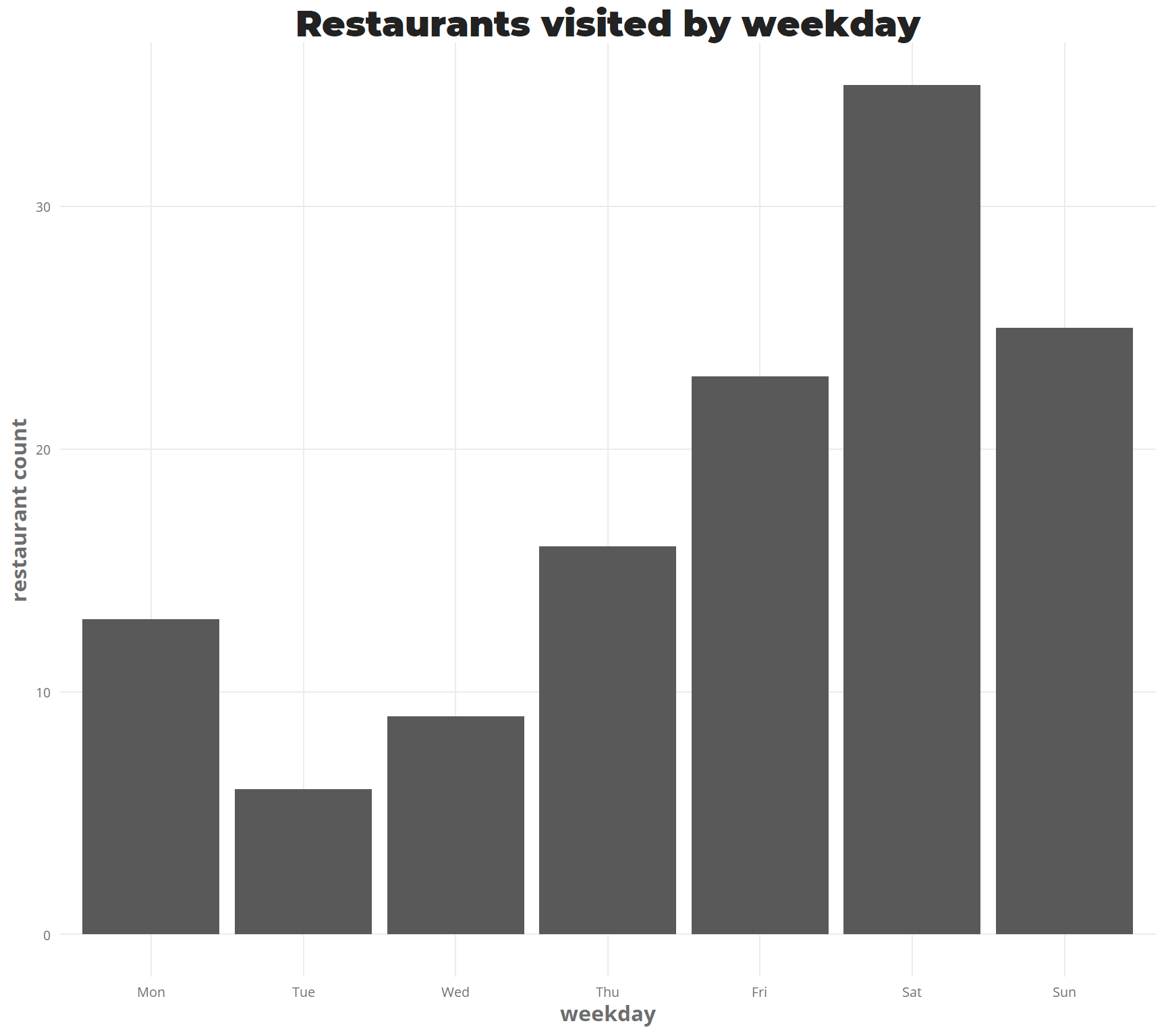
At the same time summer and winter vacations are the best time to try new restaurants.
To visualize it more clearly, we will first take the months where I have had an expense on a restaurant not in Finland (my curent home). And create a new table with a column stating if I have been abroad or not.
month_abroad <- restaurants %>%
  filter(country != "Finland") %>%
  pull(month) %>%
  unique()

restaurants_month <- restaurants %>%
  group_by(month) %>%
  summarize(n = n()) %>%
  mutate(abroad = ifelse(month %in% month_abroad,"abroad","home"))
We can then easily plot it, August and December, the period with the longest vacations are the ones that have had the biggest visits to restaurants.
ggplot(restaurants_month) +
  geom_col(mapping = aes(month,n,fill = abroad)) +
  labs(title = "Restaurants visited by month",
    y = "restaurant count",
    fill = "")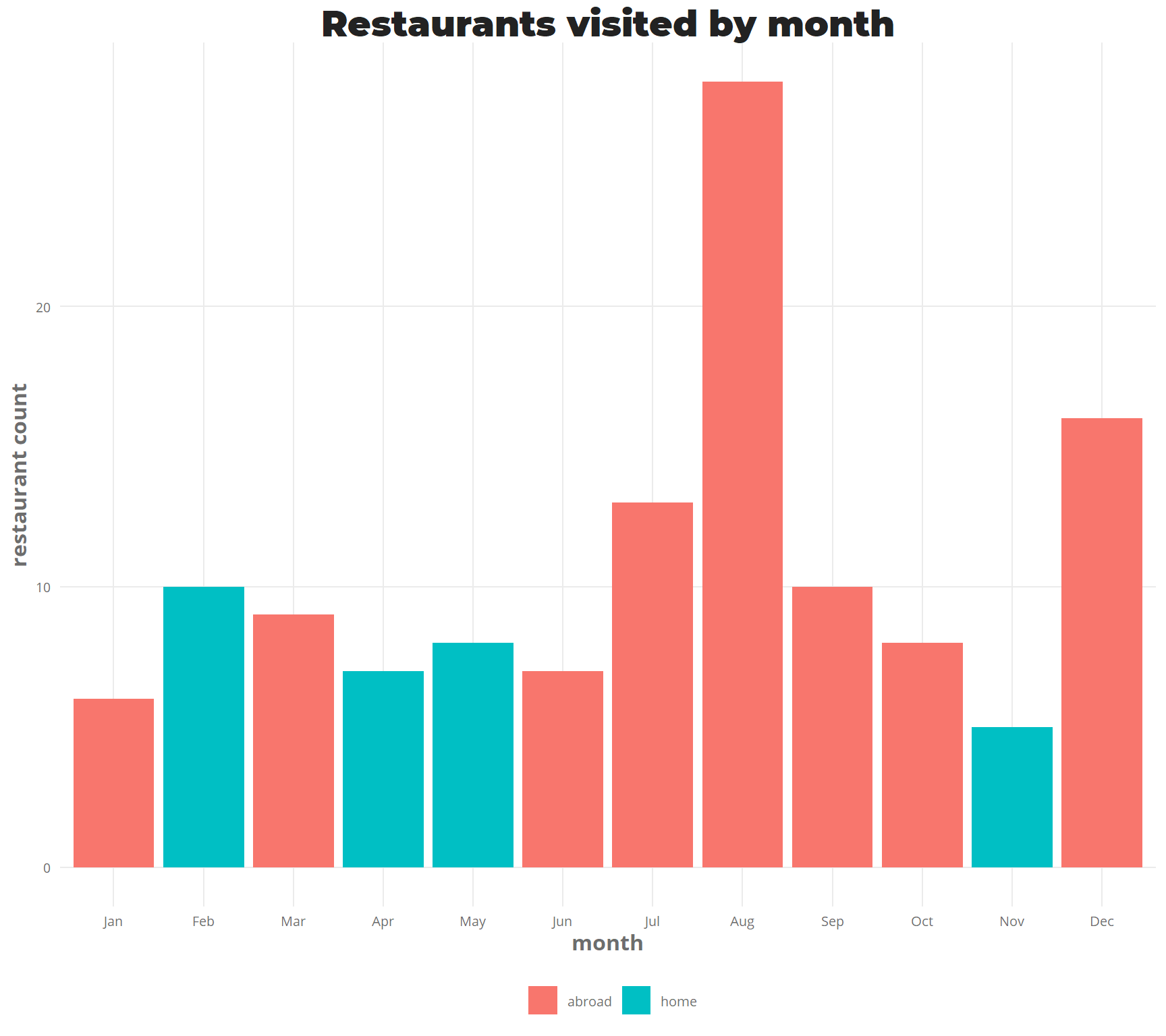
Restaurant types
I have assigned a category to each restaurant, which is quite a difficult task due to the diversity of the restaurants visited, and to avoid too big fragmentation, some of them have been put together. Idea is to understand how much I have spent in total for each of the categories, and how much is the median money spent per restaurant in that category.
restaurants %>%
  group_by(restaurant_type) %>%
  summarize(total_spent = sum(amount_eur),
    median_per_restaurant = median(amount_eur),
    count = n()) %>%
  ggplot() +
  geom_col(mapping = aes(x = fct_reorder(restaurant_type,total_spent,.desc = FALSE),
    y = total_spent,
    fill = median_per_restaurant)) +
    coord_flip() +
  scale_fill_gradient(trans = "log10",low = "light blue",high = "dark blue") +
  labs(title = "Restaurants spenditure by food type",
    x = "Restaurant type",
    y = "Total spent in EUR",
    fill = "median cost \n (EUR)")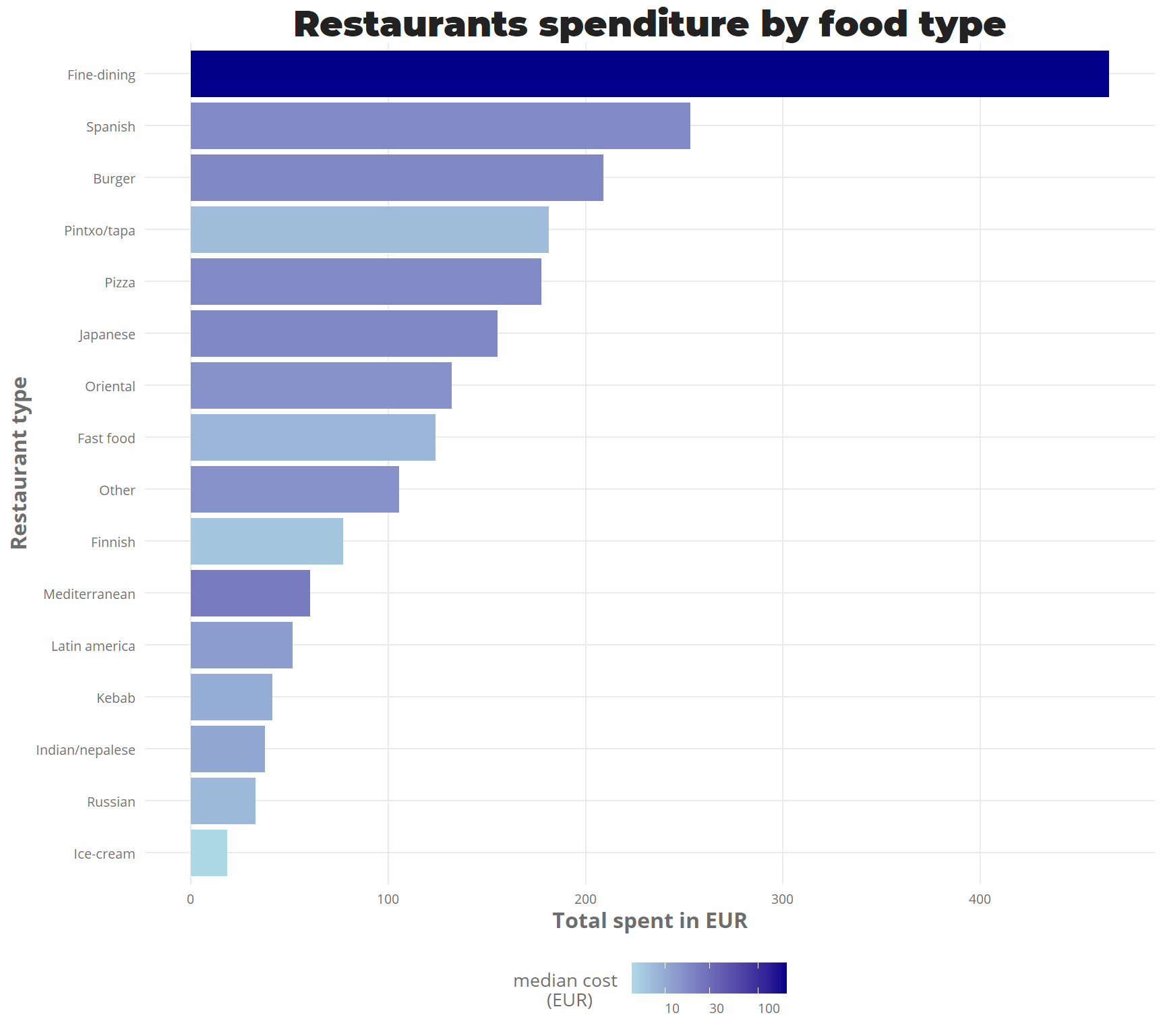
Visiting as little as 3 fine-dining restaurants, brings these to the top category, where most money has been spent. However the experience in asador Etxebarri on January was totally worth the money and one of the best culinary experiences I will ever have.
Work cantine is considered as Finnish restaurant type, thus the low median cost, as the lunch there costs only between 4-6 euros. Something interesting is that even if the Pintxo/tapa category has a very low median cost, it ranks to 4th in the categories where I have spent most money, indicating that I have been in a lot of such restaurants/bars.
Also special mention to ice-cream that even if it could not be considered as a restaurant type, is one of my favourite desserts, and everytime I go to Tallinn I try to visit Cortile for an amazing Italian ice cream.
Habits by country
While I have been in multiple countries trying food, only in 3 of them I have been in more than 10 restaurants along the 12 last months. As I am curious about the differences in spenditure among these countries, I decided to calculate the percentage of restaurants that are within different cost groups:
- 0 to 10 euros
- 10 to 20 euros
- 20 to 50 euros
- 50 to 220 euros
For this analysis, workplace restaurant is excluded, as I have been there quite a lot of times and that would skew the data in Finland percentages.
countries_over_10_restaurants <- restaurant_summary %>%
  group_by(country) %>%
  summarize(n = n()) %>%
  filter( n > 10) %>%
  pull(country)


restaurants %>%
  filter(country %in% countries_over_10_restaurants,
    restaurant_name != "Rosmariini (work)") %>%
    mutate(cost_group = santoku::chop(amount_eur,c(0,10,20,50,220))) %>%
  group_by(cost_group,country) %>%
  summarize(n = n()) %>%
  group_by(country) %>%
  mutate(total_country = sum(n) ,
    percentage = (n/total_country)*100) %>%
  select(country,cost_group,percentage) %>%
  spread(cost_group,percentage) %>%
  kable() %>%
kable_styling(bootstrap_options = "striped", full_width = F)| country | [0, 10) | [10, 20) | [20, 50) | [50, 220] |
|---|---|---|---|---|
| Estonia | 31.25000 | 56.25000 | 12.50000 | NA |
| Finland | 32.75862 | 31.03448 | 31.03448 | 5.172414 |
| Spain | 35.71429 | 39.28571 | 17.85714 | 7.142857 |
It is interesting to see, how well balanced is the mix between different categories for Finnish restaurants, being the country where I live in I try to balance cheaper options together with regular and fancier restaurants. However when going to Estonia, I try to avoid more very cheap restaurants, as for a bit more I can get good quality restaurants for a reasonable price, specially when comparing to Finland.
Interactive restaurant map
Thanks to the library leaflet, it is very easy to show all this restaurants in an interactive map with just few lines of code
jechave_tiles <- paste0("https://api.mapbox.com/styles/v1/kutteb/ck9h39xng0png1iqyyvmqchpb/tiles/256/{z}/{x}/{y}@2x?access_token=",keyring::key_get("mapbox_token",keyring = "jechaveR"))
mb_attribution <- " <a href='https://www.mapbox.com/map-feedback/'>Mapbox</a>  <a href='http://www.openstreetmap.org/copyright'>OpenStreetMap</a>"

rest_map <- leaflet(data = restaurant_summary,height = 500) %>%
    addTiles(urlTemplate = jechave_tiles, attribution = mb_attribution) %>%
   addMarkers(~long,~lat,popup = ~restaurant_name,
    clusterOptions = markerClusterOptions())
saveWidget(rest_map, here::here("static","html_maps","restaurants_last_12m.html"))